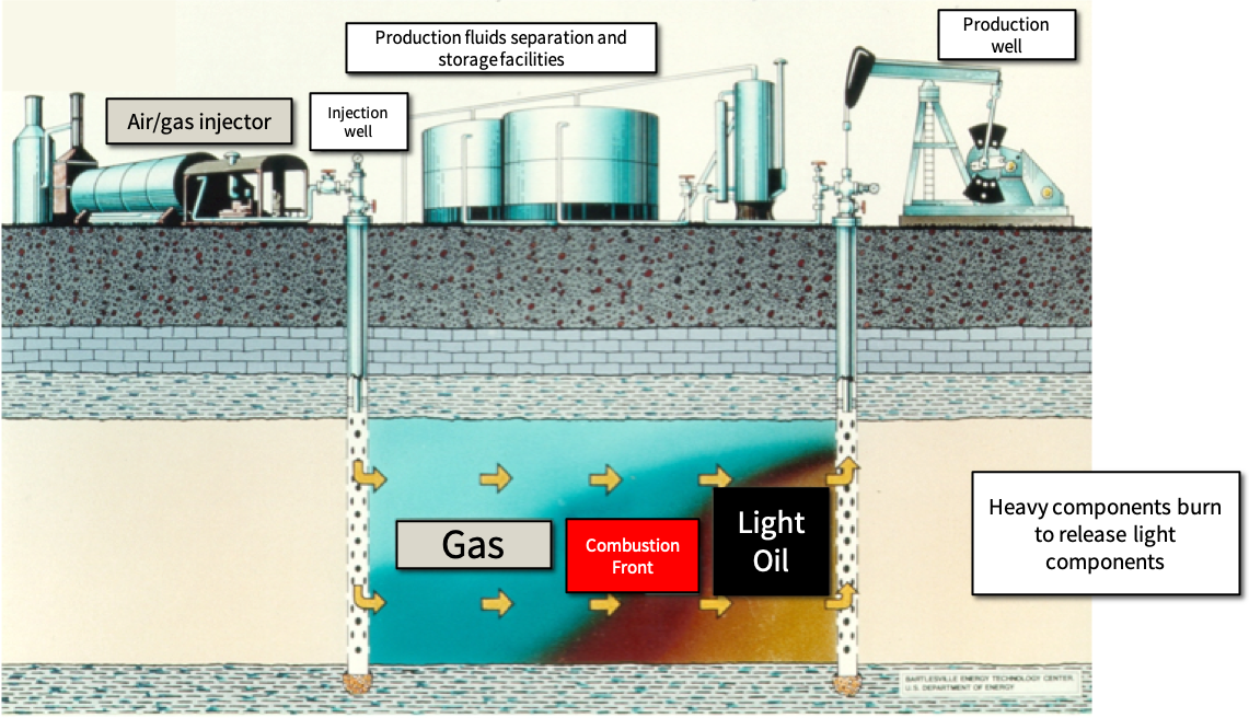
Enhanced oil recovery (EOR) typically involves applying heat, pressure, or a chemical solvent to a reservoir to increase the amount of oil recovered. In-situ combustion (ISC) is a form of thermal EOR where instead of injecting an external source of heat and/or pressure (e.g. steam), air is injected into the reservoir and the oil is burned in place. Lighter components of the oil are mobilized and pushed ahead of the combustion front where they are eventually recovered at the extraction well, while heavier components stay behind and burn:
Calibrating Reaction Models
One of the biggest questions for ISC is how does oil burn? Oil is very chemically complex, so we can’t actually model every single reaction taking place. Instead, we choose to model oil burning as a series of reactions with hydrocarbon pseudocomponents e.g.:
\[\begin{align*} \text{Oil} + \text{O}_2 &\rightarrow \text{Oil}_2 + \text{H}_2\text{O} \\ \text{Oil}_2 &\rightarrow \text{Coke} + \text{CO}_2 \\ \text{Oil}_2 + \text{O}_2 &\rightarrow \text{CO} + \text{CO}_2 + \text{H}_2\text{O} \\ \text{Coke} + \text{O}_2 &\rightarrow \text{CO} + \text{CO}_2 \end{align*}\]This gives us a simplified chemical reaction model which we can upscale to reservoir-scale simulations of ISC. To obtain a useful model, we need to fit the kinetics parameters (stoichiometric coefficients, activation energies, etc.) to match experimental data obtained from burning oil in a controlled laboratory setting.
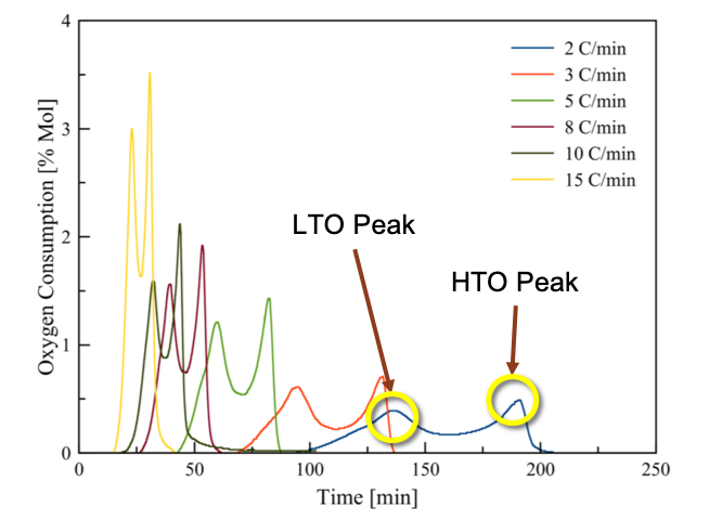
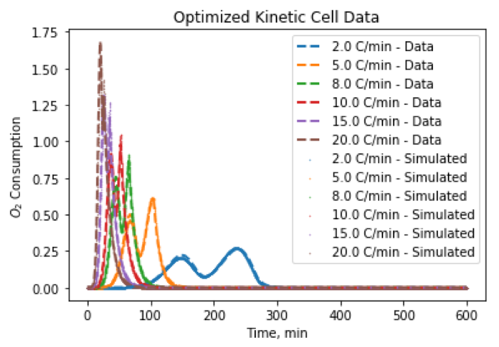
My research explores three challenges in calibrating ISC reactions:
- How do we efficiently calibrate parameters to experimental data and quantify uncertainty in these matched parameters?
- What is the relationship between a reaction scheme’s structure and its ability to fit ISC data?
- How can we determine the best reaction scheme to describe a given oil sample?
The goal is to obtain a simplified but descriptive chemical reaction model for petroleum combustion that eventually can be upscaled to a reservoir-scale simulation of ISC. Work in this area is ongoing, although results for this project will be published in the near future.
Predicting Kinetics Directly from Laboratory Data
One way we can track the progress of an ISC reaction is examining the oxygen conversion, or the proportion of total oxygen that has been reacted at time \(t\):
\[\begin{align*} C_{\text{O}_2} = \frac{\int_0^t ([\text{O}_2]_{\text{in}} - [\text{O}_2](\tau)) d\tau}{\int_0^\infty ([\text{O}_2]_{\text{in}} - [\text{O}_2](\tau)) d\tau} \end{align*}\]An idea we have explored is predicting \(\text{O}_2\) conversion curves using a data driven model. Using the fact that \(\text{O}_2\) conversion rate is independent of the time \(t\), we can model the conversion rate \(C_{\text{O}_2}'\) as only a function of the temperature \(T\) and the current \(\text{O}_2\) conversion:
\[\begin{align*} C_{\text{O}_2}' = f(T, C_{\text{O}_2}) \end{align*}\]This predictive model can then be used with an ODE solver to generate conversion curves for an input temperature schedule.
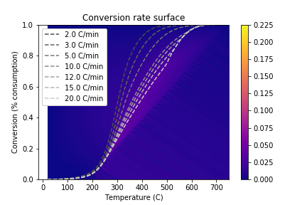
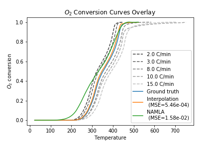
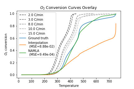
Previous work in our lab has used a linear interpolation or lookup table approach for the model \(f(T, C_{\text{O}_2})\). However, these methods are unable to capture combustion dynamics at query points outside the range of experimental data. To overcome this challenge, we proposed to use locally-weighted linear regression to predict the consumption rate at a given query point. The nonparametric regression model allows us to reconstruct the entire consumption rate surface, including points for high temperature/low consumption that are undefined with an interpolation approach:
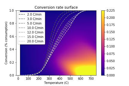
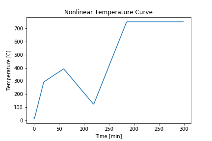
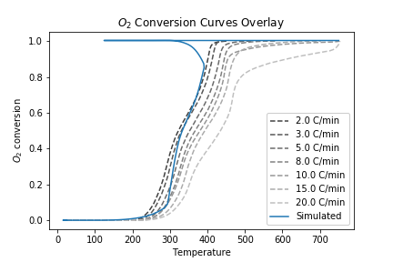
This allows us to simulate temperature schedules that lie outside the range of experimentally-observed \((T, C_{\text{O}_2}, C_{\text{O}_2}')\) values:
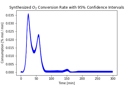
An additional advantage of the regression approach is that we can quantify uncertainty in the predicted values:
Our hope is that this work will allow us to create synthetic \(\text{O}_2\) consumption curves which can be used to improve fitting kinetics parameters to pseudocomponent chemical reaction models.

