
Takeaways
- We derive the differential equation governing the displacement of each mass in our system using Newton’s second law: \[F_{net} = \underbrace{\sum_i F_i}_{\text{All forces acting on mass}} = ma = m x’’\] and solve the resulting equations using the characteristic equation and undetermined coefficients methods.
- The equation of motion for a spring is Hooke’s Law: \[F = -k x\]
- The equation of motion for a dashpot is: \[ F = -\beta v = -\beta x’ \]
Overview
The last portion of CME 102 is focused mainly on applications of the material we’ve learned: we’ve teased applications here and there, but the focus has been solidly on the mathematics. Now that we’ve learned the bulk of the math (or enough of it), it’s time to transition to doing more applications.
The first (and most important) one of these is mass-spring systems. You’re probably asking yourself, why do we care so much about mass-spring systems? We study these systems because a huge range of engineering problems can be modeled as/reduced down to simple mass-spring systems. A couple of these include:
- Mechanical systems involving masses and springs (duh)
- Solid mechanics systems: each small section of a solid material can be modeled as a spring or with damping
- Fluid flow: mass-spring models are actually the starting point for deriving the equations of motion for fluids
- Circuits: as you’ll see in the next section of notes, circuits actually follow a very similar form to mass-spring systems
- There’s actually something called a mechanical computer which uses mass-spring systems instead of electrical circuits to perform computation
- Quantum mechanical systems: the connection is pretty complicated, and I’ll leave it at that
If it makes you feel any better, back when I took this class the importance of mass-spring systems was also completely lost on me. Hopefully providing a little motivation here at the start will help you trudge through the remainder of this page.
In what follows, we’ll first go over the basic components of a mass spring system, and how to set up the equations. From there, we’ll go through a few cases of oscillations, and point out the characteristic properties of each one.
Equations of Motion: Springs, Dashpots, and Newton’s Second Law
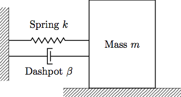
Mass spring systems are composed of three main components: masses, springs, and dashpots. We use the equations for the spring and friction (dashpot) forces in conjunction with Newton’s second law to create the equation(s) of motion for the system. To get the idea of what we’re talking about, let’s consider a very simple mass spring system:
Let’s start with Newton’s second law. Recall (maybe) from your physics class Newton’s second law of motion:
\[F_{net} = ma\]Here, \(a\) is the acceleration of the object, \(m\) is the mass, and \(F_{net}\) is the net force.
This law holds for any object in motion. What is basically says is that the net force acting on an object (i.e. if we went through and tallied up everything pushing/pulling the object) is equal to the mass of the object times its acceleration. Force and acceleration are a vector quantities, so this law holds for each component (dimension) of the vector. Fortunately for us though, in this section (and in CME 102) we’ll only be looking at motion along one dimension, so we do not need to worry about vectors.
Another way of writing Newton’s section law is:
\[\sum_i F_i = ma\]where we’ve explicitly written the net force as a sum of all the forces acting on the object. This equation will become the equation of motion, but first we need to figure out what the \(F_i\) are in the sum.
Springs: The first force is the spring force. We can write the force exerted on a mass \(m\) at position \(X\) (note that this is a big \(X\)) as:
\[F_{spring} = -k \underbrace{\Delta X}_{\text{displacement}}\]That is, the force exerted by a spring is equal to the change in stretch of the spring times the spring constant \(k\). (This is just Hooke’s law, for those of you who remember it from physics. But if you don’t, that’s cool too.)
Now for something confusing: notice here that we’ve written the spring force in terms of the change in absolute position from some sort of reference. However, what is this reference? How do we figure out what \(\Delta X\) is? Well, the fact is that we don’t really need to know the absolute position, we just need to know the displacement from equilibrium.
To do this, let \(x(t) = X(t) - X_{equilibrium}\). We know that there exists some sort of equilibrium position \(X_{equilibrium}\), and some absolute position \(X\), but we don’t know what these are, and sometimes we don’t even have a way to know. From here on out, we’ll write all the equations of motion in terms of the displacement \(x(t)\) (lower case x). Doing this, we can rewrite Hooke’s Law as:
\[F_{spring} = -k x\]That is, the force is always in the opposite direction of the displacement (e.g. if mass moves to the left, the force exerted by the spring points to the left). One thing people get hung up on is the sign of \(x(t)\)—that is, if the \(x(t)\) is negative, shouldn’t we change the sign of the force? While this is a bit confusing, the fact is that we do not care about the sign of the displacement, we only care about the sign of the force relative to the displacement. In the above equation, the force is defined to be opposite the direction of the displacement, so we’re set.
Dashpots: Next we need to write the equation for a dashpost. What’s a dashpot, you ask? Great question! A dashpot is basically just an object that we use to represent friction. The force from a dashpot is given by:
\[F_{dashpot} = -\beta v\]where \(v\) is the velocity of the object. That is, the force from the dashpot is always in the opposite direction of motion, and proportional to the velocity. A real life example of a dashpot is a plunger on a syringe: the faster you try to pull out the syringe, the more resistance it gives. However, in real-life systems a dashpot is just there to represent any form of friction, since friction force obeys this law.
Finally, we can write the equation of motion for the above mass-spring system. Start with Newton’s second law:
\[ma = \sum_i F_i = F_{spring} + F_{dashpot}\]Then, insert the equations for the forces:
\[ma = -kx - \beta v\]Note that the velocity \(v(t)\) and acceleration \(a(t)\) are just the first and second derivatives of the displacement \(x(t)\). So, we can write the above equation as:
\[mx'' = -kx - \beta x'\]or:
\[mx'' + \beta x' + kx = 0\]which is just a linear constant coefficient second order ODE, which we are already very familiar with.
Solving Equations of Motion for Mass-Spring Systems
While the physics behind mass-spring systems may seem difficult at first, you’ve fortunately already studied the differential equations that govern their motion. Mass spring systems in this class will always lead to a linear second order constant coefficient ODE. If we are only dealing with one mass, we’ll only have one equation; if there are multiple masses, we’ll have one equation for each mass.
The general flow for solving mass-spring system problems is:
- Derive the equation(s) of motion for the system by using Newton’s second law (applied separately to each mass).
- Combine terms and put into standard form. The ODEs will always be linear, second order, and have constant coefficients.
- Solve using the methods we have already learned (usually characteristic equation and undetermined coefficients).
In the remainder of this page, we’ll look through a few cases related to mass-spring systems. As you go through these, keep this workflow in mind, and also be sure to try to relate the equations of motion back to one of the solution methods we’ve already learned. Specifically, we will be using the characteristic equation to solve the homogeneous/unforced equations, and undetermined coefficients to solve systems with external force applied to at least one mass in the system.
Free Oscillations
The simplest type of mass-spring system is free oscillaiton, or undamped motion. This means that there is no damping/friction present in the system. Consider the simple system below:
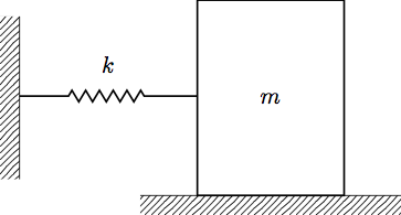
The equation of motion for this system is:
\[mx'' = -kx\]So the solution is:
\[x(t) = C_1 \sin\left(\sqrt{\frac{k}{m}}t\right) + C_2 \cos\left(\sqrt{\frac{k}{m}}t\right)\]Clearly, all undamped motion will be a sinusoidal solution. If we think back to the characteristic equation solution to the above ODE, undamped motion always has two conjugate, pure imaginary roots, which means the solution will always be a sinusoid.
Damping
We now move on to damped motion. Damped motion is exactly what it sounds like: you have damping in the system i.e. there is a dashpot or other source of friction in the system. As an example, let’s look at the example from the beginning of this section of notes:
We already saw that the equation of motion for the mass is:
\[mx'' + \beta x' + kx = 0\]Before we go further, let’s rewrite this equation a bit so it will be in a more general form. We want to make the equation look like:
\[x'' + 2 \mu x' + \omega^2 x = 0\]For this ODE, we can do this by substituting \(\lambda = \frac{\beta}{2m}\) and \(\omega^2 = \frac{k}{m}\). Whenever you have a mass spring system, you should always put the ODE in this form, since it will make it much easier to identify the below cases for damping.
Now that we’ve rearranged the equation, we can easily solve using the characteristic equation \(x(t) = Ce^{\lambda t}\). This yields:
\[\lambda = -\mu \pm \sqrt{\mu^2 - \omega^2}\]This should look very familiar to when we were classifying solutions with characteristic equation (since we’re essentially doing this again). There are three main cases for damped (unforced) motion:
- Overdamped motion: \(\omega^2 < \mu^2\) (two distinct, real roots) which has solution: \(\begin{gather} x(t) = C_1 e^{(-\mu + \sqrt{\mu^2 - \omega^2})t} + C_2 e^{(-\mu - \sqrt{\mu^2 - \omega^2})t} \end{gather}\)
- Critically damped: \(\omega^2 = \mu^2\) (one real, repeated root) \(\begin{gather} x(t) = e^{-\mu t}(C_1 + C_2 t) \end{gather}\)
- Underdamped: \(\omega^2 > \mu^2\) (two complex conjugate roots) \(\begin{gather} x(t) = e^{-\mu t} \left[ C_1 \cos\left(\sqrt{\omega^2 - \mu^2} t\right) + C_2 \sin \left(\sqrt{\omega^2 - \mu^2}t\right) \right] \end{gather}\)
Examples of these types of motion are shown in the plot below:
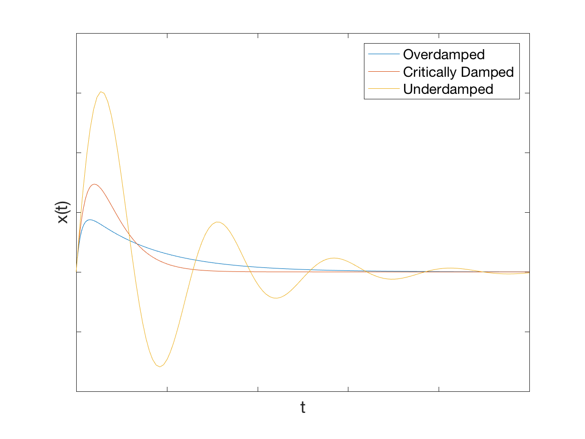
Notice that overdamped and critically damped motion look pretty similar, but are very different from underdamped motion. Underdamped motion will always be a decaying sinusoid, and therefore is easy to identify.
Note: you should be able to match equations to plots for mass-spring systems. A central part of doing so is having intuition for how the plot looks for each type of mass-spring system.
Multiple Springs and Dashpots
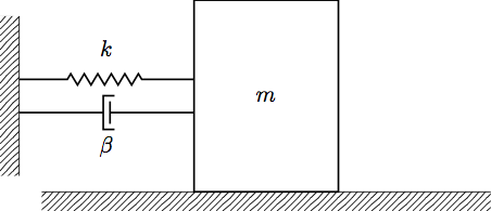
Before we move onto the hard section, we should quickly note what happens when we have multiple springs/dashpots in a system. Consider the mass-spring diagram below:
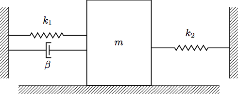
Whenever we have multiple springs/dashpots, we follow the same procedure as before: write the force balance equation, then rearrange to be in standard form. For this system:
\[\begin{gather} mx'' = -k_1 x - \beta x' - k_2 x \\ m x'' + \beta x' + (k_1 + k_2 )x = 0 \end{gather}\]Notice that when we have multiple springs or dashpots, all of the damping terms and spring constants will group together with \(x'\) and \(x\), respectively.
What if we have springs in series or parallel? Consider the mass-spring system below:
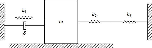
Here, we have two springs in parallel, so we need to group these springs together:
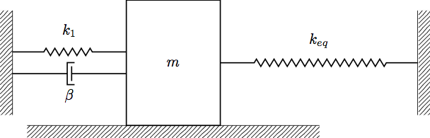
Notice that this looks just like the diagram from the beginning of the mulitple springs/dashpots section, so if we know all of the spring constants (i.e. can find \(k_{eq}\)), we already know the equation of motion. Springs in parallel obey a similar rule as resistors in parallel, i.e.
\[\frac{1}{k_{eq}} = \frac{1}{k_1} + \frac{1}{k_2}\]So for this system, we have:
\[k_{eq} = \frac{k_2k_3}{k_2 + k_3}\]Using this, we can easily write the equation of motion for the mass.
Forcing, Beats, and Resonance
Now we come to forced mass-spring systems. Forced motion means there is some sort of outside force acting on the masses (i.e. motion independent of the spring or damping forces). Let’s modify the above mass-spring system slightly to include a forcing term i.e. something driving the mass that is driven separately from the mass:
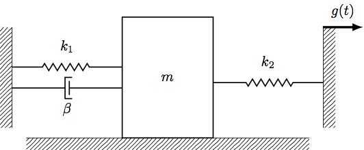
This is the same mass-spring system from before, but we’ve added a platform connected to \(m\) with spring that moves according to some function \(g(t)\). To derive the equation of motion for \(m\), we once again start with the force balance equation:
\[\begin{align} ma &= \sum_i F_i \\ &= F_{\text{spring 1}} + F_{\text{dashpot}} + F_{\text{spring 2}} \\ mx'' &= - k_1 x - \beta x' + F_{\text{spring 2}} \end{align}\]Now we just need to treat the force term from the second spring. We can write the equation for the force from a spring (regardless of whether the endpoints are moving or not) as:
\[F_{\text{spring}} = - k \Delta L\]where \(L(t)\) is the length of the spring. Now, we could go through in gory detail how to arrive at this, but I know most of you don’t really care, so I’m just going to give you the result. For a spring acting on a mass \(m\), we can write the force from the spring as:
\[F_{\text{spring}} = - k \left([\text{Displacement of mass}] - [\text{Displacement of other endpoint}] \right)\]Notice that this equation actually generalizes the equation when the opposite end point was fixed—if the opposite end point is attached to a wall i.e. fixed, there is no displacement. (As an aside, this is the same idea we’ll use when deriving equations for multi-degree of freedom systems below.)
Using this, we can write the force from the second spring above as:
\[F_{\text{spring 2}} = - k_2 (x - g(t))\]so the equation of motion becomes:
\[mx'' = - k_1 x - \beta x' - k_2 (x - g(t))\]or
\[mx'' + \beta x' + (k_1 + k_2)x = k_2 g(t)\]So, a forcing function will just give us an inhomogeneous linear second order constant coefficient ODE.
Before we go any further, let’s recall that generalized form of the mass-spring equation, and add in a forcing term:
\[x'' + 2 \lambda x' + \omega^2 = r(t)\]Now we have something pretty general that will be easy to work with. Typically, the forcing function will be on oscillatory function i.e. a sine or a cosine, so \(r(t)\) will look something like:
\[r(t) = F_0 \sin(\gamma t)\](It could also have a cosine, but to keep our lives easier, we’ll just stick with a sine. Notice though that all the results remain the same even if the forcing function was a cosine.)
There’s four cases of forced mass-spring systems that we care about:
- When the system is damped (and therefore has a decaying homogeneous solution)
- When the system is undamped and its natural frequency \(\omega\) is very different from the forcing frequency \(\gamma\)
- Undamped and \(\omega \approx \gamma\)
- Undamped and \(\omega = \gamma\)
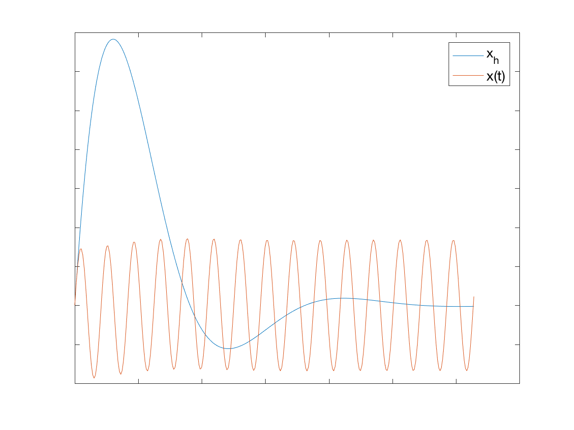
Case 1 (damped motion): The first case is pretty simple. When we have damping, we know that the homogeneous solution will be a decaying sinusoid, and from method of undetermined coefficients we know that the particular solution will be a sine/cosine. (See how undetermined coefficients is coming back here?) The homogeneous solution decays over time, so it is known as the transient solution. The particular solution is just a sine or cosine, which goes on forever, so it’s known as the steady state solution. (In general, when you hear “steady state solution”, you should immediately think about what the solution looks like as \(t \to \infty\).)
For Case 1, a sample solution is shown in the plot below. Notice how the solution is a superposition of the homogeneous and particular solutions, and the homogeneous solution decays over time.
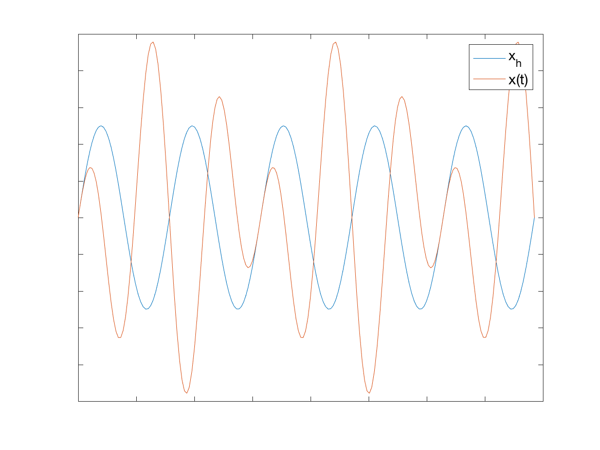
Case 2 (undumped and \(\omega \neq \gamma\)): Case 2 is pretty similar to the first, except we have no damping (i.e. \(\lambda=0\)), and consequently both the homogeneous and particular solutions do not decay (they are both sinusoids with distinct frequencies). Consider the example in the plot below. Notice that the solution is a superposition of two sinusoids.
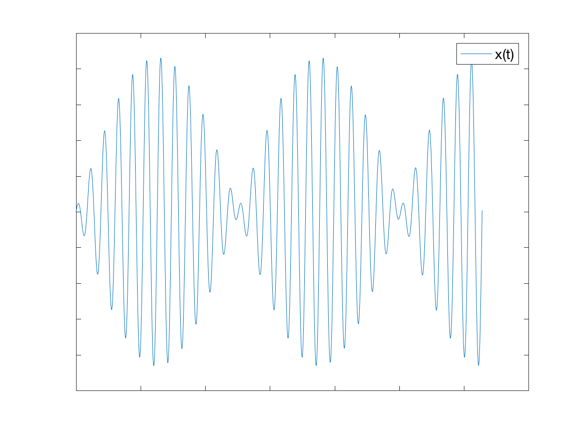
Case 3 (undamped with \(\omega \approx \gamma\)): Case 3 is known as beats. This is where \(\omega \approx \gamma\) and there’s no damping, so both the homogeneous and particular solutions are sinusoids and we have cancellation between the homogeneous and particular solutions. An example solution is shown in the plot below. It is actually possible to show that when \(\omega \approx \gamma\), the solution will be a superposition of two sine waves with very similar frequencies, but this requires a lot of algebra to show and isn’t going to significantly improve your life, so we don’t go into it here.
Case 4 (undamped with \(\omega = \gamma\)): Finally, we have Case 4. This case is known as resonance, and occurs when \(\omega=\gamma\) and we have no damping. Recall that for an ODE of the form:
\[x'' + \omega^2x = F_0 \sin(\omega t)\]the particular solution is
\[x_h(t) = C_1 \sin(\omega t) + C_2 \cos(\omega t)\]To solve for the particular solution, we use method of undetermined coefficients. However, \(r(t)\) here matches the homogeneous basis functions, so we need to apply the modification rule. Therefore, the particular solution will be of the form:
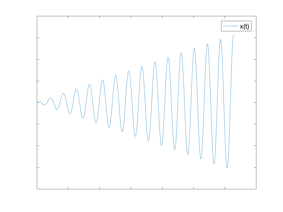
\[x_p(t) = A t \sin(\omega t) + B t \cos(\omega t)\]So, we see that the particular solution grows in time. (You can think of it as a sine/cosine with the amplitude growing in time.) This is why when we have resonance, the solution blows up. An example of resonance is shown in the plot below. When looking at a plot of a solution, it is easy to spot resonance because the solution will always be growing linearly in \(t\).
I know that was a lot, but hopefully you got through it unscathed. This last section should be pretty easy in comparison.
Multi-Degree of Freedom Systems
Finally, we have multi-degree of freedom (multi-DoF) mass-spring systems. While these look daunting at first, we’ll see that we’ve actually done most of the hard work already. Let’s start with a simple (forced) multi-DoF mass-spring system:
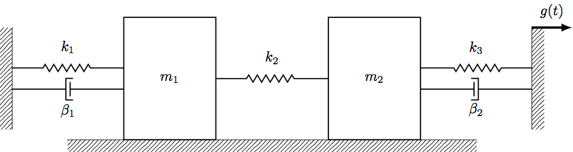
When we have a multi-DoF systems, we need to write a force balance equation for each mass (each DoF). Intuitively this makes sense: we have two independent functions we need to solve for, so we’ll need one differential equations for each.
Let’s start by writing the equation for Mass 1. To do this, we begin with Newton’s second law:
\[m_1 x_1'' = -k_1 x_1 - \beta_1 x_1' - k_2[\text{Stretch on spring 2}]\]Remember from above when both end points of the spring are moving, we calculate the stretch as the difference between the displacement of the mass and the displacement of the other end. In this case, the other end is the displacement of Mass 2. So, the equation of motion for Mass 1 is:
\[m_1 x_1'' = -k_1 x_1 - \beta_1 x_1' - k_2(x_1 - x_2)\]Similarly for Mass 2, we use Newton’s second law to write the equation of motion. Note here that we have a dashpot with two moving ends. The force from the dashpot will be opposite the direction of the net velocity. So, very similarly to the spring force, we calculate net velocity as velocity of the mass minus velocity of the other end. We can then write the equation of motion as follows:
\[m_2 x_2'' = -k_2 (x_2 - x_1) - k_3(x_2 - g(t)) - \beta_2(x_2' - g'(t))\]See? Not too bad.
Concluding Remarks
The most important thing to takeaway about mass-spring systems is the qualitative characteristics of the solutions instead of the actual analytical solutions. All mass-spring system equations will boil down to linear second order constant coefficient ODEs, which we’ve already learned how to solve in great depth. The power of analyzing systems in terms of mass-spring systems is being able to model a system and quickly determine if we’ll have resonance, beats, a particular type of damping, etc. This type of analysis is far more valuable for engineering systems than being able to derive a certain solution for a certain forcing function by hand.
Either way, just remember to start with Newton’s second law, write the force balance equation, and know how to check for the different types of motion discussed here. If you can do this, you’ll be in great shape for any mass-spring system problems you encounter.